BD-Oculars
BD-Oculars
BD-Oculars
BD-Oculars
BD-Oculars
BD-Oculars
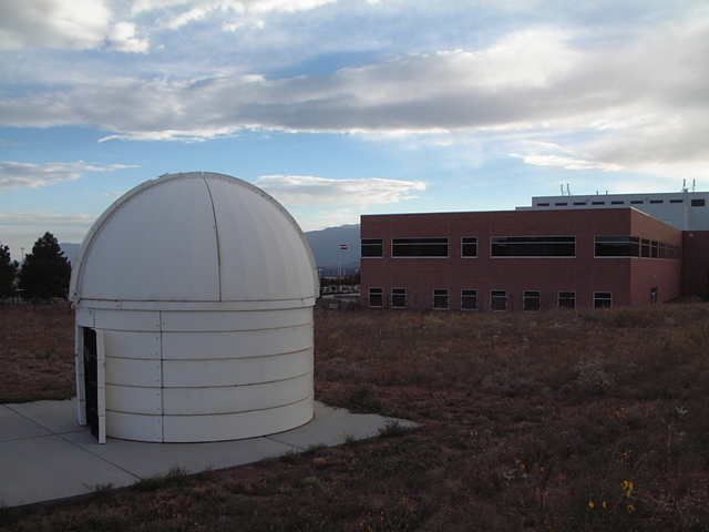
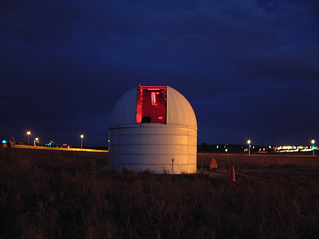
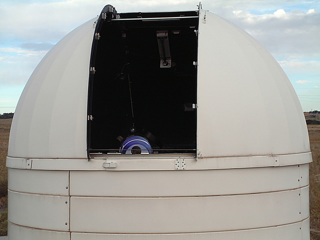
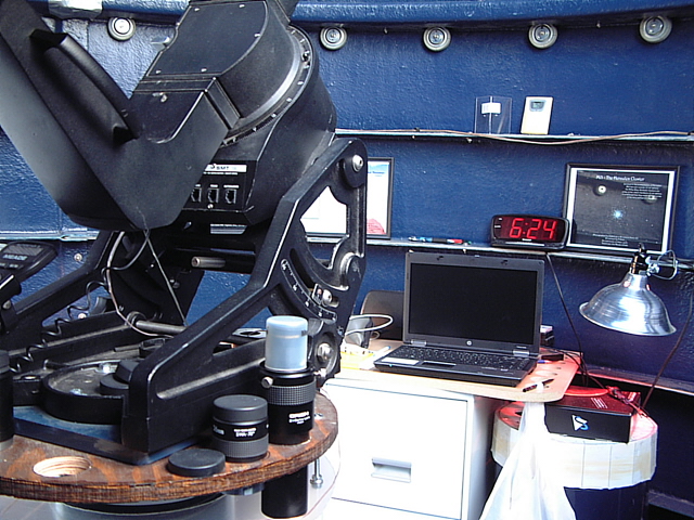
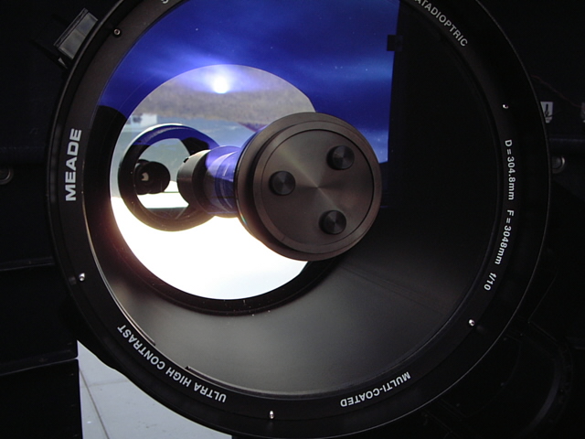
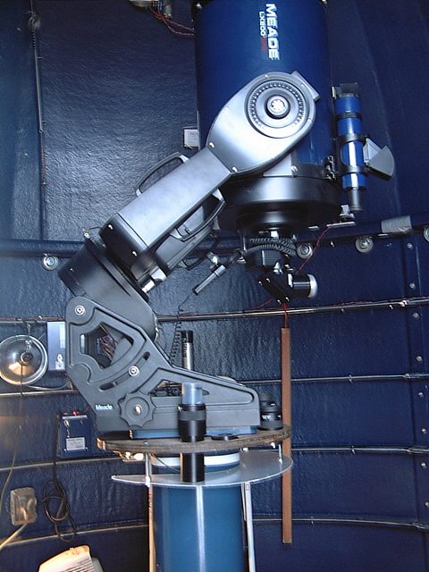
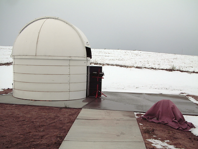
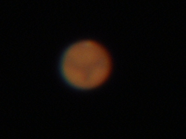
Recent changes at the Tessmer Observatory (Pikes Peak Community College) include the installation of a Bisque Software ME II mount in their new 15 ft. diameter dome.
A new telescope will be installed (16in Meade SCT).
.gif)
Previous pictures of the old 10ft. diameter dome (no longer present).

OPTICS
A grinding machine in action!
 Click on the picture to see a movie of a grinding machine in action.
MAX and MIN eyepiece
Here is an easy way to calculate the maximum and minimum size eyepiece that will work with any telescope. First, determine the F-ratio of your telescope:
{This is the focal length divided by the diameter of the primary.}
MIN Magnification:
Multiply the F-ratio by six (6). {This gives you the maximum eyepiece focal length (in millimeters). This is the lowest power eyepiece you should use with this telescope.}
MAX Magnification:
Divide the F-ratio value by two (F#/2). {This is the minimum eyepiece focal length (maximum power).} Any eyepiece with a focal length smaller than this will exceed the upper limit of useful magnification {usually determined by multiplying the diameter of your objective (in inches) by 50}
Easy enough to remember, huh?
EXAMPLE:
Your primary mirror is eight(8) inches wide; and it has an 80 inch focal length (pretty long!).
So, your telescope is an f-10. Your maximum useable eyepiece focal length would be 60mm (from 10x6=60). And the highest power eyepiece you should use would be a 5mm focal length (from f-10/2=5). This telescope will use a wide range of eyepieces. But, nothing less than 5mm is worth trying if the conditions are short of spectacular.
This can help you save $$ [by not buying eyepieces which won't work on your telescope] and time.
Try using it for your telescope and eyepieces (maybe at a star party - using other eyepieces beyond the limit?!).
Why does this work?
Because:
MAGNIFICATION=(Entrance Pupil)/(Exit Pupil)
And:
MAGNIFICATION=(Telescope Focal Length)/(Eyepiece Focal Length)
When the two formulas are combined (since Mag1=Mag2); we get:
(Entrance)/(Exit)=(Telescope FL)/(E.P. FL)
or, (E.P. FL)=(Exit)*{(Telescope FL)/(Entrance)}
Which boils down to... (E.P. FL)=(Exit)*(F-ratio)
Entrance Pupil = your telescope's largest diameter (ie - the objective lens/mirror)
Exit Pupil = your eye's widest diameter {typically 6mm}
The nice part is this works for any telescope!
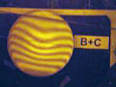
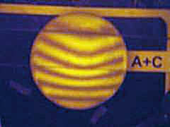
- Flats
Some 6-inch Flats that I made:
The background light is monochromatic (sodium line). Using an interferometer, you may "see" the flatness between two mirrors. Between each interference line there is 1/2-wavelength of seperation between the two surfaces. This causes a "topographic relief map" of the combination to appear.
You can think of flats as mirrors with infinite focal length. However most flats do not have focal lengths quite that long. The focal length will depend on whether the average surface departure is convex or concave, and the diameter of the mirror. It is easier (and more correct) to grade a flat by the amount that it's surface departs from being flat in degrees of wavelength (for the given color used to test the flat).
The surface of mirror "C" was within 1/16 wave of being flat; "A" was 1/8 wave; and "B" was nearly 1/4 wave. This describes the average surface "flatness". With the proper test equipment, mirrors of extremely small surface errors (1/20-wavelength or less) may be measured.
By equating their relative interference patterns to equations {A + B = %-of-half-wave, etc.}; it is possible to build a matrix to solve for the three surfaces in terms of their percentage of a half wavelength.
This was a really fun project, but it took me forever to finish the flats. It was a lesson in patience and thought.
- The MTF
Click on the first picture for additional info.
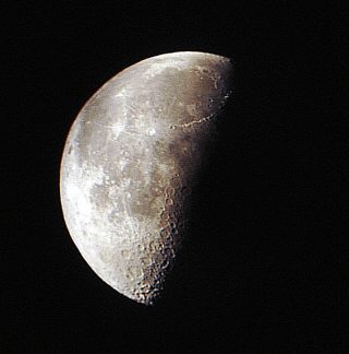
Third Quarter Moon:
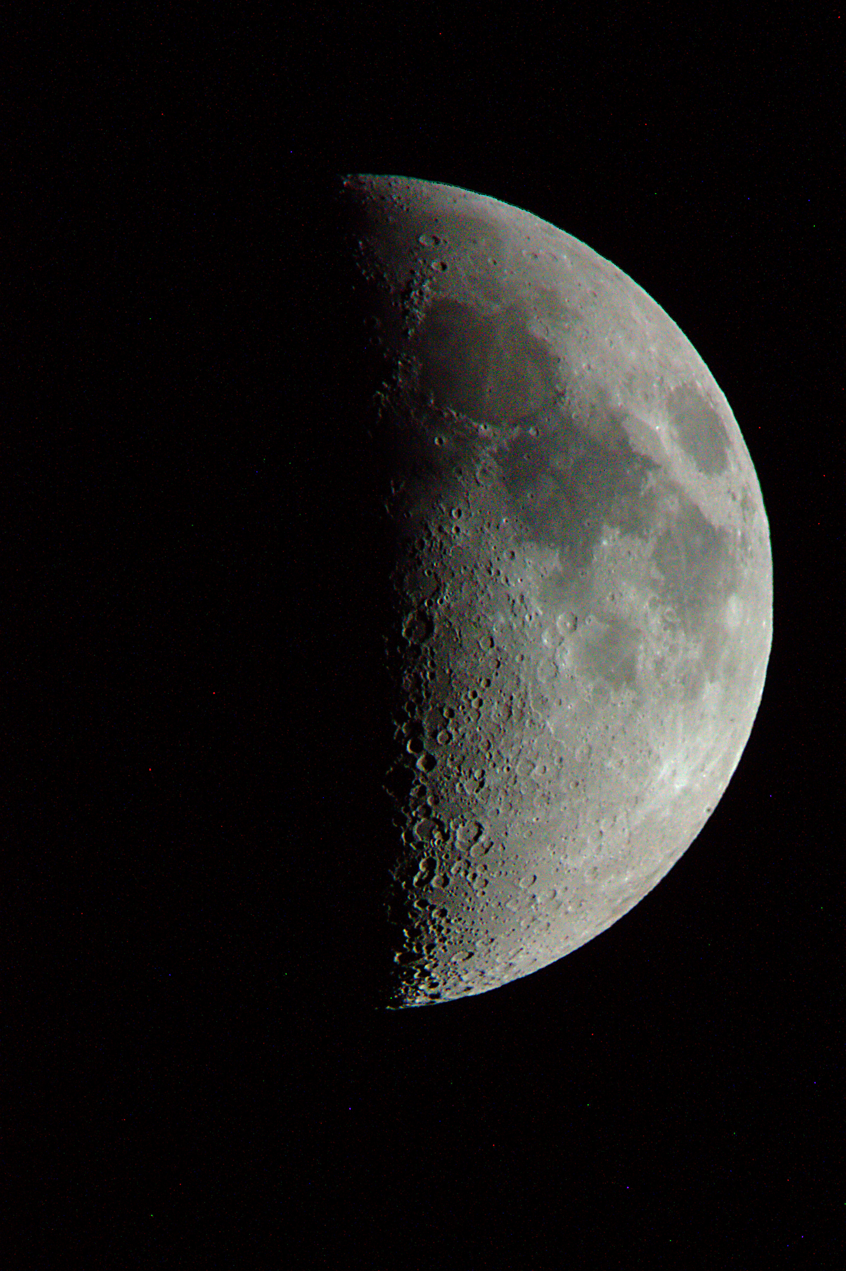
First Quarter Moon: Telescope - 60mm refractor, Camera - Canon Rebel, Post-Processing - UFRaw & GIMP
An MTF (Modulation Transfer Function) is a fancy way to show you how your optics will perform (or not) if you were to look at a test pattern of alternating white and black stripes. This is confusingly called "CYCLES/MM" in the graph. I have set the scale so that each increment represents 1000 alternations per inch (or 39.37 Cyc./MM).
As you can see, the telescope image on axis will pass 50% of it's image past the 2000 Alt/in. While the off axis image (in this case the outter edge of Saturn - dia.=20arcsec) will easily pass 50% of that image at a resolution of 500 Alt/in. The typical human retina will be able to resolve the entire image (it usually starts in the lower left hand corner and arcs upward to cross the "perfect" line at 50% - which occurs near 3000 Alt/in.) If you simplify this and draw a straight line from the lower left corner to the midpoint of the "perfect" line you will find that the outter image edge will pass above the 1000 Alt/in. mark; and should be resolved by the typical retina. For a very nice explanation of this go to:
http://www.normankoren.com/Tutorials/MTF.html
- The TFMTF
The TFMTF (Thru Focus MTF) graph is another way to confirm what the SPOT graph shows. The transfer is 90%+ for "on axis" image as well as the "outter edge" image at " zero focus". As in the SPOT graph, I have made the IN and OUT focus range +/- 1/4-inch.